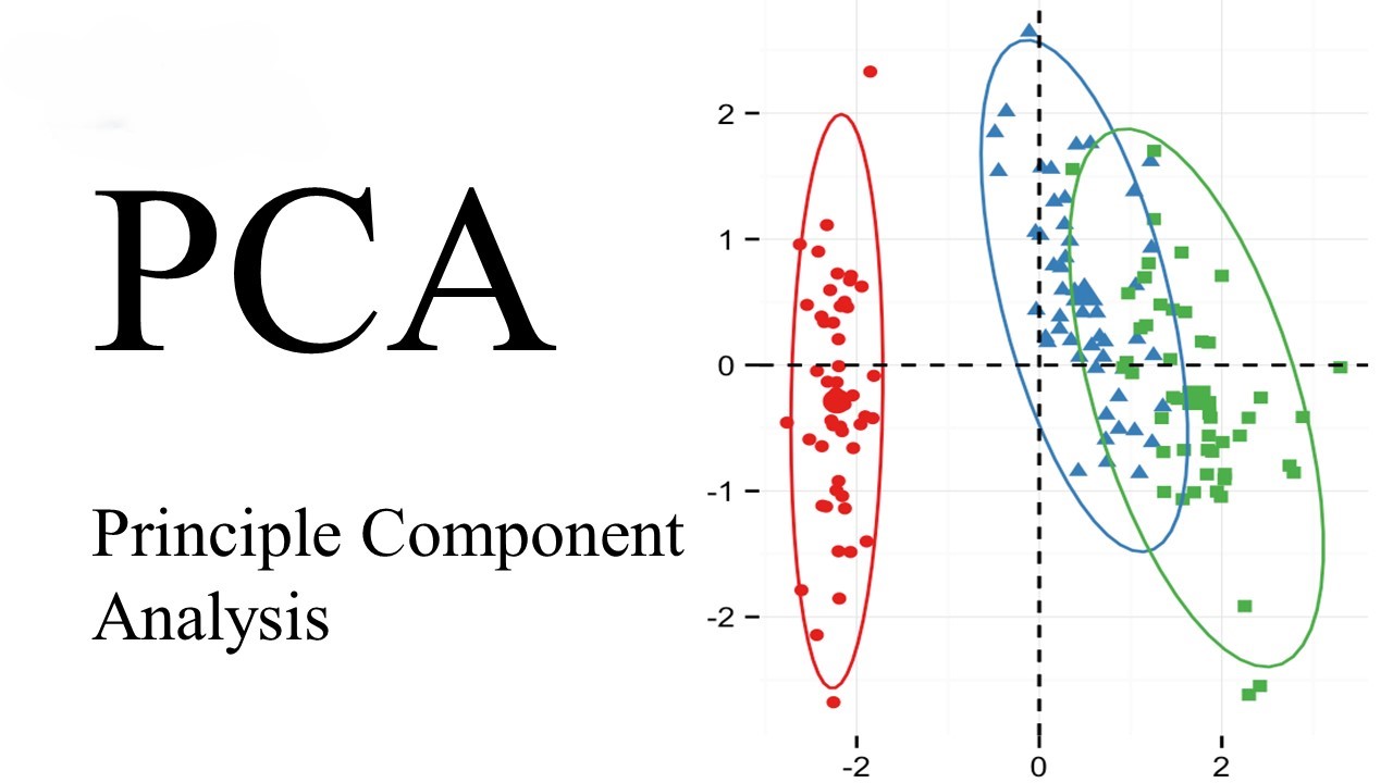
Introduction
In the vast landscape of machine learning, we’ve delved into supervised learning methods for predicting labels based on labeled training data. Now, let’s embark on a journey into the realm of unsupervised learning. Here, the focus is on algorithms that uncover intriguing aspects of data without relying on any known labels. One such workhorse in the unsupervised domain is Principal Component Analysis (PCA).
Introducing Principal Component Analysis
At its core, PCA is a nimble and speedy unsupervised method designed for dimensionality reduction. However, its utility extends beyond that, encompassing visualization, noise filtering, feature extraction, and more. In this exploration, we’ll dissect the PCA algorithm conceptually and dive into practical examples that showcase its versatility.
#Standard import
s%matplotlib inline
import numpy as np
import matplotlib.pyplot as plt
import seaborn as sns; sns.set()
Understanding the Basics of PCA
To grasp the essence of PCA, let’s first visualize its behavior using a two-dimensional dataset. Consider a set of 200 points, and let’s find the principal axes using Scikit-Learn’s PCA estimator.
rng = np.random.RandomState(1)
X = np.dot(rng.rand(2, 2), rng.randn(2, 200)).T
plt.scatter(X[:, 0], X[:, 1])
plt.axis('equal')
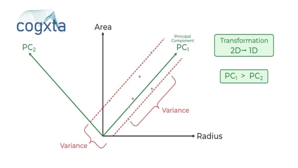
Unveiling Principal Components
PCA quantifies the relationship between variables by identifying principal axes and their corresponding explained variance. These components, as vectors, showcase the importance of each axis in describing the dataset.
from sklearn.decomposition import PCA
pca = PCA(n_components=2)
pca.fit(X)
print(pca.components_)
print(pca.explained_variance_)
Visualizing Principal Components
Visualizing principal components as vectors over the input data provides insights into their significance. These vectors, representing the axes, unveil the variance of the data when projected onto each axis.
def draw_vector(v0, v1, ax=None):
ax = ax or plt.gca()
arrowprops=dict(arrowstyle='->', linewidth=2, shrinkA=0, shrinkB=0)
ax.annotate('', v1, v0, arrowprops=arrowprops)
#Plot data and principal
componentsplt.scatter(X[:, 0], X[:, 1], alpha=0.2)
for length, vector in zip(pca.explained_variance_, pca.components_):
v = vector * 3 * np.sqrt(length)
draw_vector(pca.mean_, pca.mean_ + v)
plt.axis('equal')PCA for Dimensionality Reduction
Utilizing PCA for dimensionality reduction involves eliminating less important principal components. The transformed data, in a reduced dimension, preserves the maximal data variance.
pca = PCA(n_components=1)
pca.fit(X)
X_pca = pca.transform(X)
print("original shape: ", X.shape)
print("transformed shape:", X_pca.shape)
Visualizing Dimensionality Reduction
To understand the impact of dimensionality reduction, we can perform the inverse transform and plot the results alongside the original data.
X_new = pca.inverse_transform(X_pca)
plt.scatter(X[:, 0], X[:, 1], alpha=0.2)
plt.scatter(X_new[:, 0], X_new[:, 1], alpha=0.8)
plt.axis('equal')
PCA for Visualization: Hand-written Digits
The true potential of dimensionality reduction becomes apparent in high-dimensional datasets. Applying PCA to the digits dataset, a 64-dimensional space representing 8×8 pixel images, demonstrates its efficacy in visualization.
from sklearn.datasets import load_digits
pca = PCA(2)
projected = pca.fit_transform(load_digits().data)plt.scatter(projected[:, 0], projected[:, 1], c=load_digits().target, edgecolor='none', alpha=0.5, cmap=plt.cm.get_cmap('spectral', 10))
plt.xlabel('component 1')
plt.ylabel('component 2')
plt.colorbar()
Understanding the Components
Going beyond visualization, PCA helps us interpret the reduced dimensions in terms of basis vectors. By understanding the role of basis functions, PCA enables us to efficiently represent data in a lower-dimensional space.
Choosing the Number of Components
Estimating the optimal number of components is vital in PCA. Examining the cumulative explained variance ratio guides us in selecting the right balance between dimensionality reduction and information preservation.
pca = PCA().fit(load_digits().data)
plt.plot(np.cumsum(pca.explained_variance_ratio_))
plt.xlabel('number of components')
plt.ylabel('cumulative explained variance')
PCA as Noise Filtering
PCA doubles as a noise filtering tool. By reconstructing data using the largest subset of principal components, we retain the signal while discarding noise.
# Generating noise-free and noisy data
noisy = np.random.normal(load_digits().data, 4)

# Training PCA on noisy data
pca = PCA(0.50).fit(noisy)
components = pca.transform(noisy)
filtered = pca.inverse_transform(components)
Example: Eigenfaces
Exploring PCA’s role in feature selection, we revisit facial recognition using eigenfaces. Leveraging PCA, we significantly reduce dimensionality while preserving essential facial features.
from sklearn.datasets import fetch_lfw_people
from sklearn.decomposition import RandomizedPCA
faces = fetch_lfw_people(min_faces_per_person=60)
pca = RandomizedPCA(150).fit(faces.data)
components = pca.transform(faces.data)
projected = pca.inverse_transform(components)Wrapping Up PCA
Principal Component Analysis proves to be a versatile unsupervised learning method with applications in dimensionality reduction, visualization, noise filtering, and feature selection. Its interpretability and efficiency make it a powerful tool for gaining insights into high-dimensional data. While not universally applicable, PCA offers an efficient pathway to understanding complex datasets.
In the upcoming sections, we’ll explore additional unsupervised learning methods building upon PCA’s foundational ideas. Stay tuned for more insights into the fascinating world of machine learning!
Leave a Reply