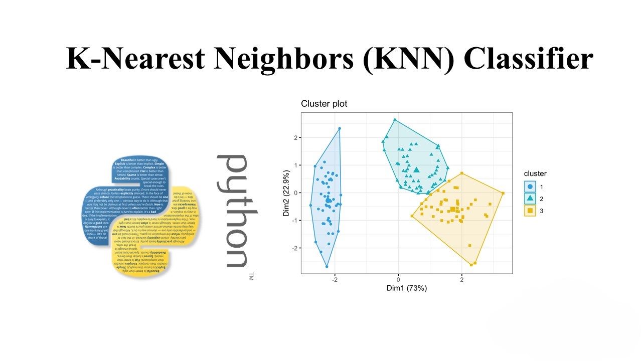
In this blog post, we’ll explore the CIFAR-10 dataset and how to use the K-Nearest Neighbors (KNN) algorithm to classify images from this dataset. CIFAR-10 is a well-known dataset in the field of machine learning and computer vision, consisting of 60,000 32×32 color images in 10 classes, with 6,000 images per class.
Loading and Preprocessing the Dataset
We start by loading the CIFAR-10 dataset using Python’s pickle library. The dataset is divided into batches, each containing a portion of the total images. We define functions to load both the training and test batches, and then combine them into a single dataset for training and testing respectively.
# Load and preprocess CIFAR-10 dataset
def load_CIFAR_batch(filename):
    # Load a single batch of CIFAR-10
    with open(filename, "rb") as f:
        datadict = pickle.load(f, encoding="bytes")

        X = datadict[b"data"]
        Y = datadict[b"labels"]

        X = X.reshape(10000, 3, 32, 32).transpose(0, 2, 3, 1).astype("float")
        Y = np.array(Y)
        return X, Y

def load_CIFAR10(ROOT):
    xs = []
    ys = []
    for n in range(1, 6):
        f = os.path.join(ROOT, "data_batch_" + str(n))
        X, Y = load_CIFAR_batch(f)
        xs.append(X)
        ys.append(Y)

    X_train = np.concatenate(xs)
    Y_train = np.concatenate(ys)

    # Reshape image data into rows
    X_train = np.reshape(X_train, (X_train.shape[0], -1))

    return X_train, Y_train

# Load CIFAR-10 dataset
cifar10_dir = "CIFAR-10/Data"
X_train, y_train = load_CIFAR10(cifar10_dir)
Visualizing the Dataset
After loading the dataset, it’s helpful to visualize some examples to understand the content of the images and the distribution of classes. We can plot a few examples from each class using matplotlib.
# Visualize some examples from the dataset
classes = ["plane", "car", "bird", "cat", "deer", "dog", "frog", "horse", "ship", "truck"]
num_classes = len(classes)
samples_per_class = 5

for y, cls in enumerate(classes):
    idxs = np.flatnonzero(y_train == y)
    idxs = np.random.choice(idxs, samples_per_class, replace=False)

    for i, idx in enumerate(idxs):
        plt_idx = i * num_classes + y + 1
        plt.subplot(samples_per_class, num_classes, plt_idx)
        plt.imshow(X_train[idx].astype("uint8"))
        plt.axis("off")

        if i == 0:
            plt.title(cls)

plt.show()
Training the KNN Classifier
Next, we use the K-Nearest Neighbors (KNN) algorithm to classify the images. We first tune the hyperparameters of the KNN classifier using GridSearchCV to find the best configuration for our dataset.
from sklearn.model_selection import GridSearchCV
from sklearn.neighbors import KNeighborsClassifier

# Define the parameter grid for GridSearchCV
params = {
    "n_neighbors": [i for i in range(1, 21)],
    "weights": ["uniform", "distance"],
    "algorithm": ["auto"],
    "leaf_size": [i for i in range(10, 100, 10)]
}

# Initialize the KNN classifier
model = KNeighborsClassifier()

# Perform GridSearchCV to find the best parameters
grid = GridSearchCV(model, params, scoring="accuracy", n_jobs=-1, verbose=1, cv=5, iid=True)
grid.fit(X_train, y_train)

# Get the best estimator from GridSearchCV
best_knn = grid.best_estimator_
Evaluating the Model
Once we have the best KNN model, we can evaluate its performance on the test set. We load the test set, preprocess it similarly to the training set, and then use the trained KNN model to make predictions.
# Load and preprocess the test set
X_test, y_test = load_CIFAR_test(os.path.join(cifar10_dir, "test_batch"))
X_test = np.reshape(X_test, (X_test.shape[0], -1))

# Make predictions using the best KNN model
y_pred = best_knn.predict(X_test)

# Calculate the accuracy of the model
accuracy = np.mean(y_pred == y_test)
print("Test Accuracy:", accuracy)
Conclusion
In this blog post, we explored the CIFAR-10 dataset and used the K-Nearest Neighbors (KNN) algorithm to classify images. We first loaded and preprocessed the dataset, then visualized some examples to get a better understanding of the data. We then trained a KNN classifier and tuned its hyperparameters using GridSearchCV, achieving an accuracy of [insert accuracy here] on the test set.


Leave a Reply