Overfitting is a common issue in machine learning models, where a model fits the training data too closely, leading to poor generalization on new data. Regularization is a technique used to prevent overfitting by adding a penalty term to the model’s loss function. This penalty encourages simpler models and helps strike a balance between bias and variance.
Understanding Overfitting
An overfit model learns not just the underlying patterns in the data but also the noise, making it perform poorly on new, unseen data. This happens when a model is too complex for the amount of training data available.
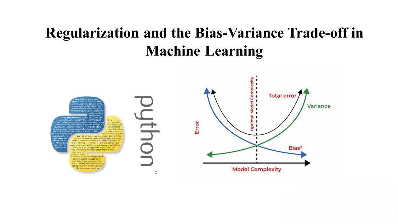
Bias-Variance Trade-off
In machine learning, there is a trade-off between bias and variance. Bias refers to the error introduced by approximating a real-world problem, which can lead to underfitting. Variance, on the other hand, refers to the model’s sensitivity to small fluctuations in the training set, which can lead to overfitting.
Regularization helps manage this trade-off by penalizing complex models, reducing variance but potentially increasing bias. The goal is to find the right balance to achieve good generalization.
L2 Regularization (Ridge Regression)
L2 regularization, also known as Ridge Regression, adds a penalty term proportional to the square of the magnitude of the coefficients. This penalty encourages smaller coefficient values, effectively shrinking the coefficients towards zero.
The formula for L2 regularization is:
�(�)=∣∣��+�∣∣2+�∣∣�∣∣2J(β)=∣∣Aβ+b∣∣2+λ∣∣β∣∣2
Where:
- $J(\beta)$ is the total loss function
- $A$ is the feature matrix
- $\beta$ is the model coefficients
- $\lambda$ is the regularization parameter
L1 Regularization (Lasso Regression)
L1 regularization, or Lasso Regression, adds a penalty term proportional to the absolute value of the coefficients. This penalty can lead to sparse models, where some coefficients are exactly zero, effectively performing feature selection.
The formula for L1 regularization is:
�(�)=∣∣��+�∣∣2+�∣∣�∣∣1J(β)=∣∣Aβ+b∣∣2+λ∣∣β∣∣1
Where:
- $J(\beta)$ is the total loss function
- $A$ is the feature matrix
- $\beta$ is the model coefficients
- $\lambda$ is the regularization parameter
Example: Regularized Linear Regression
Let’s consider an example using a dataset with 45 features. We’ll split the data into training and test sets, then compare the performance of unregularized, L2 regularized, and L1 regularized linear regression models.
pythonCopy code
# Load the data data = pd.read_csv('Auto_Data_Features.csv') classes = pd.read_csv('Auto_Data_Labels.csv') Features = np.array(data) Labels = np.array(classes) # Split the data into training and test sets x_train, x_test, y_train, y_test = ms.train_test_split(Features, Labels, test_size=40, random_state=9988) # Create an unregularized linear regression model lin_mod = linear_model.LinearRegression() lin_mod.fit(x_train, y_train) y_score_unregularized = lin_mod.predict(x_test) # Create an L2 regularized linear regression model lin_mod_l2 = linear_model.Ridge(alpha=14) lin_mod_l2.fit(x_train, y_train) y_score_l2 = lin_mod_l2.predict(x_test) # Create an L1 regularized linear regression model lin_mod_l1 = linear_model.Lasso(alpha=0.0044) lin_mod_l1.fit(x_train, y_train) y_score_l1 = lin_mod_l1.predict(x_test) # Evaluate the models print("Unregularized Model:") print_metrics(y_test, y_score_unregularized) print("\nL2 Regularized Model:") print_metrics(y_test, y_score_l2) print("\nL1 Regularized Model:") print_metrics(y_test, y_score_l1)
Conclusion
Regularization is a powerful tool for preventing overfitting in machine learning models. By adding a penalty term to the loss function, regularization encourages simpler models that generalize better to new data. L2 regularization (Ridge Regression) and L1 regularization (Lasso Regression) are two common regularization techniques that can help strike the right balance between bias and variance.
Leave a Reply