Introduction:
Linear models play a fundamental role in the field of machine learning, providing a versatile toolkit for both regression and classification tasks. In this comprehensive guide, we’ll delve into various aspects of linear models, exploring techniques for regression, classification, and addressing challenges such as outliers and non-linear relationships. Buckle up as we journey through the intricacies of linear modeling!
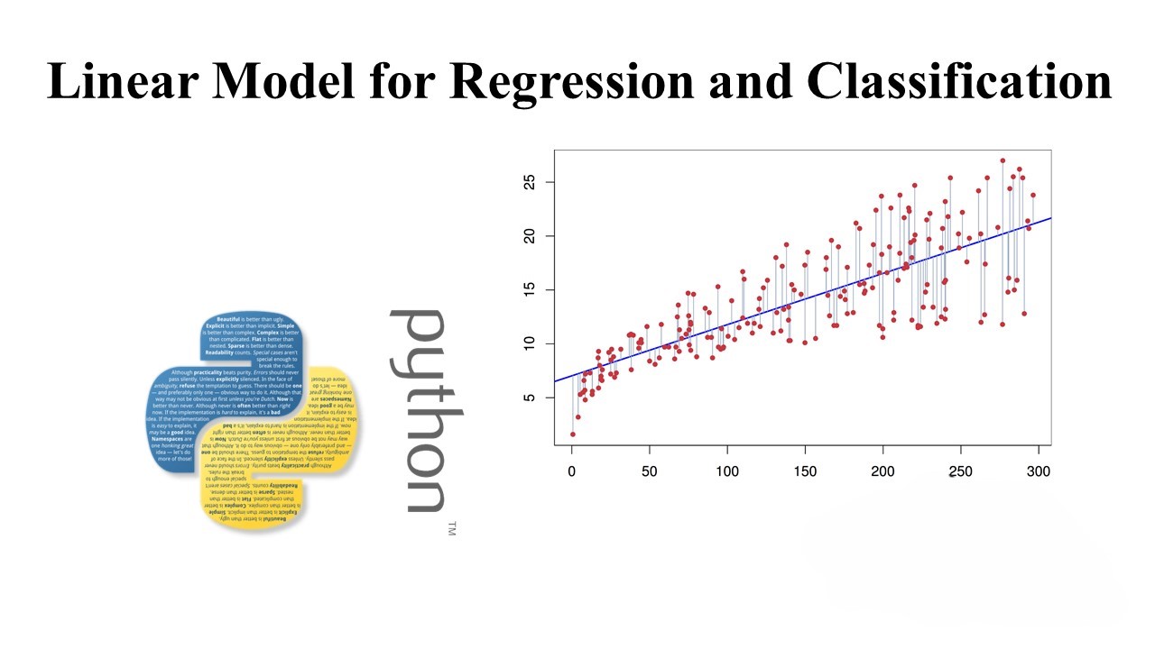
Simple Linear Regression using Ordinary Least Squares:
Let’s kick things off with the basics. Simple Linear Regression, utilizing Ordinary Least Squares, forms the foundation. We’ll explore the relationship between independent variables and the target, understanding the role of weights and intercepts in the linear equation
from sklearn.linear_model import LinearRegression
lr = LinearRegression()
lr.fit(X, Y)
Gradient Descent:
Delve into the workings of Gradient Descent, the optimization algorithm that Linear Regression employs to minimize the Residual Squared Sum (RSS) of errors. We’ll break down the mathematical underpinnings and explore how this algorithm iteratively adjusts weights to reach the optimal solution.
import numpy as np

def gradient_descent(X, Y, learning_rate=0.01, epochs=100):
    # Initialize slope and intercept
    m, b = 0, 0
    n = len(X)

    for epoch in range(epochs):
        # Calculate predictions
        Y_pred = m * X + b

        # Calculate gradients
        dm = (-2/n) * np.sum(X * (Y - Y_pred))
        db = (-2/n) * np.sum(Y - Y_pred)

        # Update parameters using gradients and learning rate
        m = m - learning_rate * dm
        b = b - learning_rate * db

        # Print the loss (Mean Squared Error) for every 10 epochs
        if epoch % 10 == 0:
            loss = np.mean((Y_pred - Y)**2)
            print(f'Epoch {epoch}, Loss: {loss:.4f}')

    return m, b

# Example usage:
X = np.array([1, 2, 3, 4, 5])
Y = np.array([2, 4, 5, 4, 5])

# Normalize data for better convergence (optional)
X = (X - np.mean(X)) / np.std(X)

# Run gradient descent
slope, intercept = gradient_descent(X, Y)

# Print the final slope and intercept
print(f'Optimal Slope (m): {slope:.4f}')
print(f'Optimal Intercept (b): {intercept:.4f}')
Regularized Regression Methods – Ridge, Lasso, ElasticNet:
To address issues like outliers and multicollinearity, we introduce regularized regression methods. Ridge Regression, Lasso Regression, and ElasticNet come to the rescue, imposing penalties on coefficients and enhancing model robustness.
from sklearn.linear_model import Ridge, Lasso, ElasticNet
ridge = Ridge(alpha=1000)
lasso = Lasso(alpha=0.1)
enet = ElasticNet(alpha=0.1)
Logistic Regression for Classification:
Linear models extend seamlessly to classification tasks with Logistic Regression. Uncover the mechanics of this algorithm, which predicts class probabilities and forms the backbone of binary classification problems.
from sklearn.linear_model import LogisticRegression
lr = LogisticRegression()
lr.fit(X, y)
Online Learning Methods – Stochastic Gradient Descent & Passive Aggressive:
For scenarios with vast datasets, online learning methods like Stochastic Gradient Descent (SGD) and Passive Aggressive algorithms shine. We’ll explore their simplicity, efficiency, and support for partial_fit in out-of-core learning.
from sklearn.linear_model import SGDClassifier
sgd = SGDClassifier(n_iter=10)
sgd.partial_fit(trainX, trainY, classes=[0, 1])
Robust Regression – Dealing with Outliers & Model Errors:
Enter the realm of robust regression, where we address the impact of outliers and model errors. Techniques such as RANSAC, Theil Sen, and HuberRegressor provide robust alternatives to standard linear regression.
from sklearn.linear_model import RANSACRegressor
ransac = RANSACRegressor()
ransac.fit(X, y)
Polynomial Regression:
When relationships are of higher polynomial degree, Polynomial Regression comes into play. We’ll demonstrate how to transform data to higher degrees and employ linear models to predict coefficients.
from sklearn.preprocessing import PolynomialFeatures
pol = PolynomialFeatures(degree=2)
X_tf = pol.fit_transform(X)
Bias-Variance Tradeoff:
Finally, we’ll explore the delicate balance between bias and variance. Understanding the Bias-Variance Tradeoff is crucial for building models that generalize well without overfitting or underfitting.
Conclusion:
As we wrap up this journey through linear models, you’ve gained insights into regression, classification, regularization, and robust techniques. Armed with this knowledge, you’re ready to tackle diverse machine learning challenges with the power of linear modeling.
Leave a Reply