Model selection and evaluation are crucial steps in the machine learning pipeline. It involves choosing the best model for a given task, tuning hyperparameters, and assessing the model’s performance. In this blog post, we will explore several aspects of model selection and evaluation, including cross-validation, hyperparameter tuning, model persistence, validation curves, and learning curves.
1. Cross-Validation
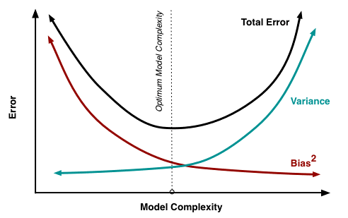
When training machine learning models, it’s essential to ensure they generalize well to unseen data. Cross-validation is a technique used to assess a model’s performance by splitting the data into multiple parts and iteratively using different subsets for training and validation. This helps in identifying whether the model is suffering from overfitting or underfitting.
Let’s consider an example using the DecisionTreeClassifier from scikit-learn on the digits dataset:
from sklearn.tree import DecisionTreeClassifier
from sklearn.datasets import load_digits
from sklearn.model_selection import train_test_split, cross_val_score

# Load digits dataset
digits = load_digits()

# Split the data into training and testing sets
trainX, testX, trainY, testY = train_test_split(digits.data, digits.target)

# Create a Decision Tree Classifier
dt = DecisionTreeClassifier(max_depth=7)

# Fit the model on training data
dt.fit(trainX, trainY)

# Evaluate on test data
test_accuracy = dt.score(testX, testY)
print("Test Accuracy:", test_accuracy)

# Cross-validate the model
cross_val_accuracy = cross_val_score(dt, digits.data, digits.target).mean()
print("Cross-Validation Accuracy:", cross_val_accuracy)
In this example, we observe how cross-validation provides a more robust estimate of the model’s performance compared to a single train-test split.
2. Hyperparameter Tuning
Models often have hyperparameters that need to be fine-tuned for optimal performance. Grid search and randomized search are common techniques for hyperparameter tuning. Here’s an example using GridSearchCV with a DecisionTreeClassifier:
from sklearn.model_selection import GridSearchCV

# Define the Decision Tree model
dt = DecisionTreeClassifier()

# Define the hyperparameters to search
param_grid = {'max_depth': range(5, 30, 5)}

# Use GridSearchCV to find the best hyperparameters
grid_search = GridSearchCV(dt, param_grid=param_grid, cv=5)
grid_search.fit(digits.data, digits.target)

# Print the best hyperparameters and corresponding accuracy
print("Best Hyperparameters:", grid_search.best_params_)
print("Best Accuracy:", grid_search.best_score_)
GridSearchCV exhaustively searches through all specified hyperparameter values, and in this example, it helps us find the optimal max_depth for the DecisionTreeClassifier.
3. Model Persistence
Once a model is trained and tuned, it’s a good practice to save it for future use. The joblib library is often preferred for model persistence. Here’s how you can save and load a trained DecisionTreeClassifier:
from sklearn.externals import joblib

# Save the model to a file
joblib.dump(dt, 'decision_tree_model.joblib')

# Load the model back
loaded_model = joblib.load('decision_tree_model.joblib')
This allows you to reuse the model without retraining, which is especially useful when working with large datasets.
4. Validation Curves
Validation curves help visualize how changing hyperparameters impacts the training and validation scores. Using scikit-learn’s validation_curve, we can plot the accuracy scores for different numbers of trees in a Random Forest model:
from sklearn.ensemble import RandomForestClassifier
from sklearn.model_selection import validation_curve

param_range = np.arange(1, 50, 2)

train_scores, test_scores = validation_curve(RandomForestClassifier(),
                                             digits.data,
                                             digits.target,
                                             param_name="n_estimators",
                                             param_range=param_range,
                                             cv=3,
                                             scoring="accuracy",
                                             n_jobs=-1)

# Plot the validation curve
# (Code for plotting not shown for brevity)
This curve helps us identify the range of hyperparameter values that yield good performance.
5. Learning Curves
Learning curves depict how a model’s performance changes with the size of the training set. This is essential for understanding whether a model would benefit from more data. Here’s a simple example using learning_curve:
from sklearn.model_selection import learning_curve

train_sizes, train_scores, test_scores = learning_curve(
    RandomForestClassifier(n_estimators=20),
    digits.data, digits.target, cv=5, n_jobs=-1)

# Plot the learning curve
# (Code for plotting not shown for brevity)
Understanding learning curves helps in determining if a model is underfitting or overfitting and whether collecting more data would be beneficial.
Conclusion
Model selection and evaluation involve various steps, including cross-validation, hyperparameter tuning, model persistence, validation curves, and learning curves. These techniques help ensure that machine learning models generalize well, perform optimally, and can be reused efficiently. By mastering these concepts, practitioners can build robust and reliable machine learning models.
Leave a Reply