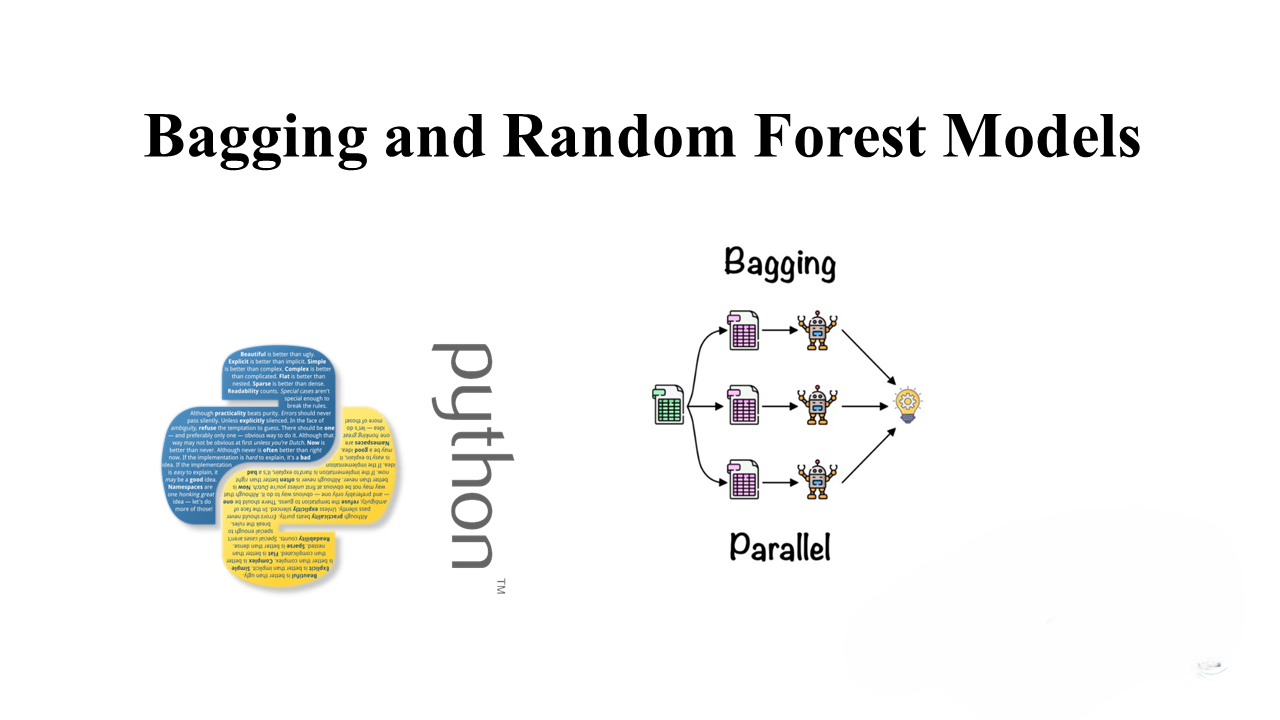
Ensemble methods are powerful techniques that combine multiple weak learners to improve predictive performance. One popular ensemble method is bagging, which aggregates the predictions of multiple models trained on subsamples of the data. Random Forest, a widely used algorithm, employs bagging with decision trees to produce robust and scalable models.
Introduction
In this blog post, we’ll explore how to use Random Forest to classify iris flower species. We’ll start by loading the necessary libraries and the iris dataset.
from sklearn.ensemble import RandomForestClassifier
from sklearn import preprocessing
import sklearn.model_selection as ms
import sklearn.metrics as sklm
import matplotlib.pyplot as plt
import pandas as pd
import numpy as np
Understanding the Iris Dataset
The iris dataset contains measurements of iris flowers’ sepal and petal dimensions, along with their species. Let’s load the dataset and take a quick look at its summary statistics.
iris = datasets.load_iris()
species = [iris.target_names[x] for x in iris.target]
iris = pd.DataFrame(iris['data'], columns=['Sepal_Length', 'Sepal_Width', 'Petal_Length', 'Petal_Width'])
iris['Species'] = species
print(iris.describe())
Preprocessing the Data
Before training the model, it’s crucial to preprocess the data. We’ll handle skewness by applying a logarithmic transformation to highly skewed features.
skew_data = iris.skew()
iris2 = iris.copy()
for c in iris2.columns[:-1]:
    if skew_data[c] > 0.3:
        iris2[c] = np.log1p(iris2[c])
Splitting the Data
We’ll split the dataset into training and testing sets, with 100 cases for testing and the rest for training.
X_train, X_test, y_train, y_test = ms.train_test_split(Features, Labels, test_size=50, random_state=123)
Scaling Features
To ensure consistent scaling, we’ll standardize the numeric features using Z-score scaling.
scale = preprocessing.StandardScaler()
scale.fit(X_train)
X_train = scale.transform(X_train)
X_test = scale.transform(X_test)
Training the Random Forest Model
We’ll define and train a Random Forest model with 10 trees.
rf_clf = RandomForestClassifier(n_estimators=10, min_samples_leaf=2, max_features='auto')
rf_clf.fit(X_train, y_train)
Evaluating Model Performance
We’ll evaluate the model’s performance using various metrics like precision, recall, and F1-score.
scores = rf_clf.predict(X_test)
print(sklm.classification_report(scores, y_test))
Visualizing Model Performance
To understand the model’s behavior, we’ll plot correctly and incorrectly classified cases.
def plot_iris_score(iris, y_test, scores):
    # Function to plot iris data by type
    # Plotting code here...

plot_iris_score(X_test, y_test, scores)
Feature Importance
Random Forest provides feature importance scores, helping identify the most influential features.
importance = rf_clf.feature_importances_
plt.bar(range(4), importance, tick_label=['Sepal_Length', 'Sepal_Width', 'Petal_Length', 'Petal_Width'])
plt.xticks(rotation=90)
plt.ylabel('Feature importance')
Conclusion
Random Forest is a versatile algorithm for classification tasks, offering robustness and scalability. By following the steps outlined in this blog post, you can effectively apply Random Forest to classify datasets like the iris dataset and achieve accurate predictions.
In future posts, we’ll explore more advanced techniques and real-world applications of ensemble learning methods like Random Forest. Stay tuned for more insights into the fascinating world of machine learning!


Leave a Reply