Support Vector Machines (SVMs) are a powerful class of supervised algorithms used for both classification and regression tasks. In this blog post, we will delve into the intuition behind SVMs and their application in solving classification problems.
Motivation
To begin, let’s consider a simple classification task with well-separated classes. We’ll generate some synthetic data with two classes using the make_blobs function from the scikit-learn library.
%matplotlib inline
import numpy as np
import matplotlib.pyplot as plt
from sklearn.datasets.samples_generator import make_blobs

X, y = make_blobs(n_samples=50, centers=2, random_state=0, cluster_std=0.60)
plt.scatter(X[:, 0], X[:, 1], c=y, s=50, cmap='autumn')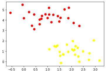
In this case, a linear discriminative classifier could draw a straight line to separate the two classes. However, there are multiple possible lines that perfectly discriminate between the classes, leading to the need for a more sophisticated approach.
Maximizing the Margin
Support Vector Machines offer a solution by introducing the concept of a margin. Instead of drawing a zero-width line, SVMs draw lines with a margin around them, up to the nearest points from each class. This margin is maximized, providing a robust classification boundary.
xfit = np.linspace(-1, 3.5)
plt.scatter(X[:, 0], X[:, 1], c=y, s=50, cmap='autumn')

for m, b, d in [(1, 0.65, 0.33), (0.5, 1.6, 0.55), (-0.2, 2.9, 0.2)]:
    yfit = m * xfit + b
    plt.plot(xfit, yfit, '-k')
    plt.fill_between(xfit, yfit - d, yfit + d, edgecolor='none', color='#AAAAAA', alpha=0.4)

plt.xlim(-1, 3.5)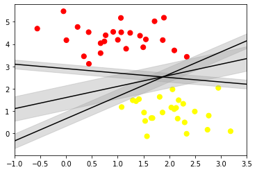
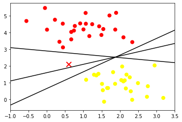
In SVMs, the line that maximizes this margin is chosen as the optimal model. Support vectors, which are the data points lying on the margin boundaries, play a crucial role in defining the decision boundary.
Fitting a Support Vector Machine
Let’s fit a support vector classifier to our data using Scikit-Learn’s SVC (Support Vector Classifier).
from sklearn.svm import SVC
model = SVC(kernel='linear')
model.fit(X, y)
The support vectors can be extracted from the model, and the decision function can be visualized.
model.support_vectors_ To visualize the decision boundary, we can use the plot_svc_decision_function function, which plots the decision boundary and support vectors.
def plot_svc_decision_function(model, ax=None, plot_support=True):
    # ... (function implementation)

plt.scatter(X[:, 0], X[:, 1], c=y, s=50, cmap='autumn')
plot_svc_decision_function(model)
Beyond Linear Boundaries: Kernel SVM
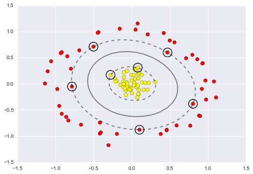
SVMs become extremely powerful when combined with kernels. Kernels allow SVMs to handle non-linear boundaries effectively. We’ll use the make_circles function to create non-linearly separable data.
from sklearn.datasets.samples_generator import make_circles
X, y = make_circles(100, factor=.1, noise=.1)

clf = SVC(kernel='linear').fit(X, y)

plt.scatter(X[:, 0], X[:, 1], c=y, s=50, cmap='autumn')
plot_svc_decision_function(clf, plot_support=False)
To handle non-linear data, we can use the radial basis function (RBF) kernel. Scikit-Learn provides an easy way to switch to the RBF kernel.
clf = SVC(kernel=’rbf’, C=1E6)
clf.fit(X, y)
plt.scatter(X[:, 0], X[:, 1], c=y, s=50, cmap=’autumn’)
plot_svc_decision_function(clf)
plt.scatter(clf.support_vectors_[:, 0], clf.support_vectors_[:, 1], s=300, lw=1, facecolors=’none’)
Tuning the SVM: Softening Margins
In real-world scenarios, data might not have a perfect separation. SVMs handle this by introducing a softening parameter C, which controls the hardness of the margin. A higher C makes the margin harder, while a lower C allows some points to enter the margin.
X, y = make_blobs(n_samples=100, centers=2, random_state=0, cluster_std=0.8)

fig, ax = plt.subplots(1, 2, figsize=(16, 6))

for axi, C in zip(ax, [10.0, 0.1]):
    model = SVC(kernel='linear', C=C).fit(X, y)
    axi.scatter(X[:, 0], X[:, 1], c=y, s=50, cmap='autumn')
    plot_svc_decision_function(model, axi)
    axi.scatter(model.support_vectors_[:, 0], model.support_vectors_[:, 1], s=300, lw=1, facecolors='none')
    axi.set_title('C = {0:.1f}'.format(C), size=14)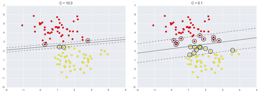
Example: Face Recognition
As a practical example, let’s explore face recognition using the Labeled Faces in the Wild dataset.
from sklearn.datasets import fetch_lfw_people
from sklearn.svm import SVC
from sklearn.decomposition import PCA
from sklearn.pipeline import make_pipeline
from sklearn.model_selection import train_test_split, GridSearchCV
from sklearn.metrics import classification_report, confusion_matrix
import seaborn as sns
import matplotlib.pyplot as plt
# Load the Labeled Faces in the Wild dataset
faces = fetch_lfw_people(min_faces_per_person=60)
# Split the data into training and testing sets
Xtrain, Xtest, ytrain, ytest = train_test_split(faces.data, faces.target, random_state=42)
# Build a pipeline with PCA and SVM
model = make_pipeline(PCA(n_components=150, whiten=True, random_state=42), SVC(kernel='rbf', class_weight='balanced'))
# Define parameter grid for grid search
param_grid = {'svc__C': [1, 5, 10, 50], 'svc__gamma': [0.0001, 0.0005, 0.001, 0.005]}
# Perform grid search to find optimal parameters
grid = GridSearchCV(model, param_grid)
grid.fit(Xtrain, ytrain)
# Get the best parameters from grid search
best_params = grid.best_params_
print("Best Parameters:", best_params)
# Use the best model to predict labels for the test set
model = grid.best_estimator_
yfit = model.predict(Xtest)
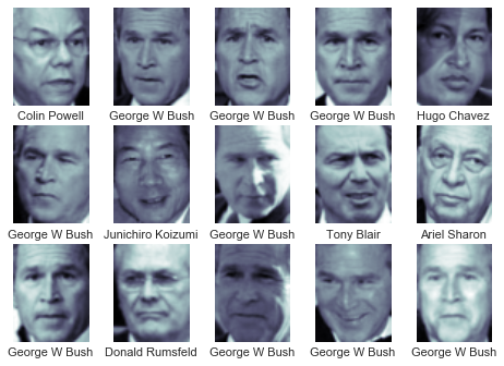
# Visualize a few test images with predicted labels
fig, ax = plt.subplots(4, 6)
for i, axi in enumerate(ax.flat):
axi.imshow(Xtest[i].reshape(62, 47), cmap='bone')
axi.set(xticks=[], yticks=[])
axi.set_ylabel(faces.target_names[yfit[i]].split()[-1], color='black' if yfit[i] == ytest[i] else 'red')
fig.suptitle('Predicted Names; Incorrect Labels in Red', size=14)
plt.show()
# Display classification report
print(classification_report(ytest, yfit, target_names=faces.target_names))
# Display confusion matrix
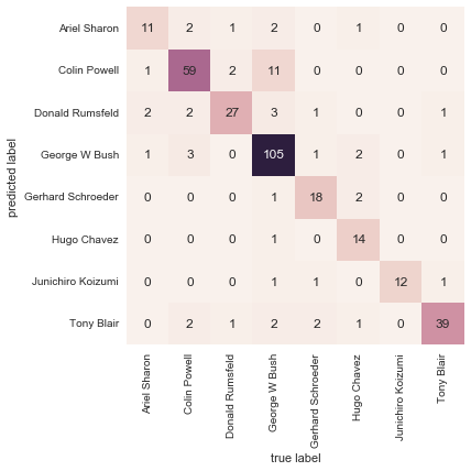
mat = confusion_matrix(ytest, yfit)
sns.heatmap(mat.T, square=True, annot=True, fmt='d', cbar=False,
xticklabels=faces.target_names, yticklabels=faces.target_names)
plt.xlabel('True Label')
plt.ylabel('Predicted Label')
plt.show()Confusion Matrix:
Precision Recall F1 score Support
Ariel Sharon 0.65 0.73 0.69 15
Colin Powell 0.81 0.87 0.84 68
Donald Rumsfeld 0.75 0.87 0.81 31
George W Bush 0.93 0.83 0.88 126
Gerhard Schroeder 0.86 0.78 0.82 23
Hugo Chavez 0.93 0.70 0.80 20
Junichiro Koizumi 0.80 1.00 0.89 12
Conclusion
Support Vector Machines are powerful tools for classification tasks, especially when dealing with high-dimensional data and non-linear boundaries. However, they come with computational costs and the need for careful parameter tuning. Understanding the principles behind SVMs and their applications allows for effective utilization in various machine learning scenarios.
About the Author:
I am Kishore Kumar K, a dedicated data scientist with a passion for unraveling insights hidden within complex datasets. With a background in MBA in Business Analytics and a BCA in Computer Applications, I have honed my skills in statistical analysis, machine learning, and data visualization. I have uploaded the blog with the guidance of Dr. Saravanapriya Manoharan.
Leave a Reply