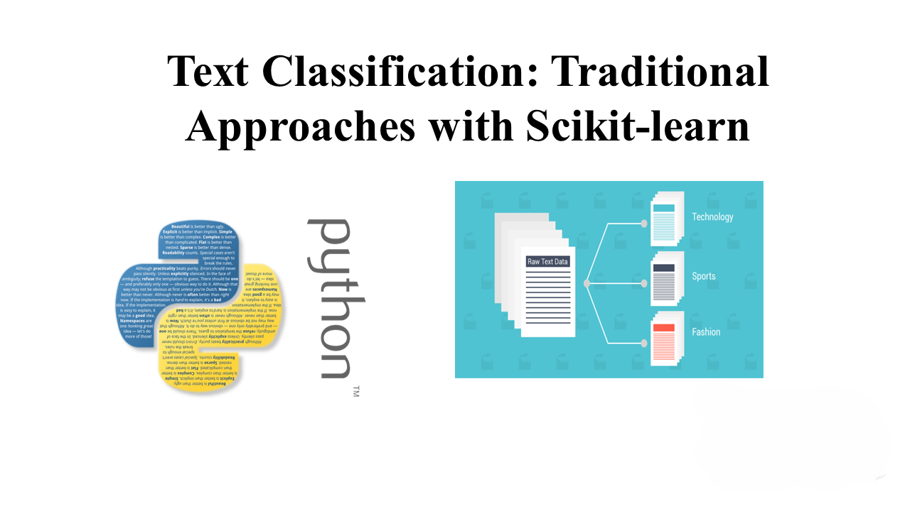
Welcome to a journey into the world of text classification, where we’ll explore some traditional yet powerful approaches using Scikit-learn. While deep learning has taken center stage in Natural Language Processing (NLP), these classical methods remain quick and effective for training text classifiers. Our playground for this experiment is the 20 Newsgroups dataset, a classic collection that spans diverse topics.
Unveiling the Dataset
Our chosen dataset, 20 Newsgroups, is a treasure trove of text documents covering an array of subjects—from computer hardware to religion. It serves as a benchmark for text classification models, with 11,314 texts for training and 7,532 for testing.
Text Preprocessing
Before we dive into modeling, let’s prepare our text data. The first step is text preprocessing, transforming raw texts into feature vectors. For this experiment, we’ll employ the “bag-of-words” approach. Scikit-learn’s CountVectorizer helps us tokenize texts and count the occurrences of each word. To add nuance, we’ll apply the Term Frequency-Inverse Document Frequency (TF-IDF) weighting, a measure that highlights words relevant to specific texts by considering their frequency in the corpus.
from sklearn.feature_extraction.text import CountVectorizer, TfidfTransformer
from sklearn.pipeline import Pipeline

preprocessing = Pipeline([
    ('vect', CountVectorizer()),
    ('tfidf', TfidfTransformer())
])

print("Preprocessing training data...")
train_preprocessed = preprocessing.fit_transform(train_data.data)

print("Preprocessing test data...")
test_preprocessed = preprocessing.transform(test_data.data)
Training the Models
With our preprocessed data in hand, it’s time to introduce our classifiers: Naive Bayes, Support Vector Machines (SVM), and Logistic Regression. Naive Bayes is simple and quick, SVM is powerful with effective separation, and Logistic Regression models the log-odds of a class as a linear model.
from sklearn.naive_bayes import MultinomialNB
from sklearn.linear_model import LogisticRegression
from sklearn.svm import LinearSVC

nb_classifier = MultinomialNB()
svm_classifier = LinearSVC()
lr_classifier = LogisticRegression(multi_class="ovr")

print("Training Naive Bayes classifier...")
nb_classifier.fit(train_preprocessed, train_data.target)

print("Training SVM classifier...")
svm_classifier.fit(train_preprocessed, train_data.target)

print("Training Logistic Regression classifier...")
lr_classifier.fit(train_preprocessed, train_data.target)
Simple Training Results
We evaluate our classifiers based on accuracy—the proportion of correct predictions. Naive Bayes achieves 77.4%, Logistic Regression 82.8%, and SVM leads with 85.3%. However, there’s room for optimization through hyperparameter tuning.
print("NB Accuracy:", np.mean(nb_predictions == test_data.target))
print("SVM Accuracy:", np.mean(svm_predictions == test_data.target))
print("LR Accuracy:", np.mean(lr_predictions == test_data.target))
Fine-tuning with Grid Search
Grid search allows us to explore hyperparameter values systematically. We focus on the $C$ hyperparameter for SVM and Logistic Regression, controlling regularization. After grid search, we discover that the default setting for SVM works best, while for Logistic Regression, increasing $C$ to 1000 yields significant improvement.
from sklearn.model_selection import GridSearchCV

parameters = {'C': [0.1, 1, 10, 100, 1000]}

print("Grid search for SVM")
svm_best = GridSearchCV(svm_classifier, parameters, cv=3, verbose=1)
svm_best.fit(train_preprocessed, train_data.target)

print("Grid search for logistic regression")
lr_best = GridSearchCV(lr_classifier, parameters, cv=3, verbose=1)
lr_best.fit(train_preprocessed, train_data.target)
Evaluating the Best Models
After grid search, we assess the performance of our refined models. Interestingly, the default SVM settings prove optimal, while Logistic Regression benefits from an increased $C$ value.
best_svm_predictions = svm_best.predict(test_preprocessed)
best_lr_predictions = lr_best.predict(test_preprocessed)

print("Best SVM Accuracy:", np.mean(best_svm_predictions == test_data.target))
print("Best LR Accuracy:", np.mean(best_lr_predictions == test_data.target))
Extensive Evaluation
Detailed Scores
Beyond accuracy, we delve into precision, recall, and F-score for each class. This comprehensive classification report reveals varying levels of difficulty for different topics.
from sklearn.metrics import classification_report, confusion_matrix

print(classification_report(test_data.target, best_svm_predictions, target_names=test_data.target_names))
Confusion Matrix
A visual representation of our model’s performance, the confusion matrix, showcases correct and misclassified predictions. It’s a valuable tool for understanding which classes are often confused.
conf_matrix = confusion_matrix(test_data.target, best_svm_predictions)
conf_matrix_df = pd.DataFrame(conf_matrix, index=test_data.target_names, columns=test_data.target_names)

plt.figure(figsize=(15, 10))
sn.heatmap(conf_matrix_df, annot=True, vmin=0, vmax=conf_matrix.max(), fmt='d', cmap="YlGnBu")
plt.yticks(rotation=0)
plt.xticks(rotation=90)
Explainability
To gain qualitative insights, we explore the features with the highest weights for each class. The library eli5 helps us interpret the SVM model, showcasing the words strongly associated with each class.
import eli5

eli5.explain_weights(svm_best.best_estimator_,
                     feature_names=preprocessing.named_steps["vect"].get_feature_names(),
                     target_names=train_data.target_names
                    )
Conclusions
In this exploration of traditional text classification, we’ve witnessed the power of Naive Bayes, SVM, and Logistic Regression. These classical methods not only serve as robust baselines but also offer deep insights into the nuances of text data. While deep learning models dominate the NLP landscape, these traditional approaches remain formidable contenders, often challenging to surpass. Through a journey into the 20 Newsgroups dataset, hyperparameter tuning, and in-depth evaluation, we’ve unraveled the art of text classification with Scikit-learn.


Leave a Reply